Version: 2.0
Status: Accepted 2025-06-01
Authors:
Implements DSEPs:
None
Description: First release of DataJoint Specs. Versioning starts with 2.0 to stay ahead of current implementations, although implementation versions are independent of the specs versions.
License
This DataJoint Specification document is licensed under the Creative Commons Attribution-ShareAlike 4.0 International License (CC BY-SA 4.0).

You are free to:
Share — copy and redistribute the material in any medium or format
Adapt — remix, transform, and build upon the material for any purpose, even commercially.
Under the following terms:
Attribution (BY) — You must give appropriate credit, provide a link to the license, and indicate if changes were made. You may do so in any reasonable manner, but not in any way that suggests the licensor endorses you or your use.
ShareAlike (SA) — If you remix, transform, or build upon the material, you must distribute your contributions under the same license as the original.
This license is available at: http://
Introduction
Purpose of DataJoint Specs
The DataJoint Specs define the standards, conventions, and best practices for designing and managing DataJoint pipelines. These specifications ensure that all DataJoint implementations remain consistent, scalable, and interoperable across various scientific workflows and computing environments.
By following the DataJoint Specs, users and developers can:
Maintain structured, reproducible data pipelines.
Ensure compatibility across different DataJoint implementations.
Adopt best practices for schema design, data integrity, and computational workflows.
Provide a foundation for future enhancements while preserving backward compatibility.
Purpose of DataJoint
DataJoint provides scientists with enhanced capabilities to design, implement, and manage the data operations underpinning their research.
At its core, DataJoint treats data and computations jointly within a formal computational database, unifying data structures and analysis code. It extends the traditional relational data model so that some tables contain raw or curated input data, while others define computations and store their results. This makes it possible to precisely construct and express entire scientific workflows—data acquisition, transformation, analysis—as structured, executable pipelines.
In this architecture, the database becomes more than just a storage system; it evolves into a living pipeline that encodes the logic and lineage of scientific work:
Structured: with explicit schema and clear data relationships
Scalable: supporting high-throughput, high-dimensional experimental data
Reproducible: with every step recorded, auditable, and rerunnable
DataJoint maintains the rigor of relational databases—ensuring data integrity, ACID-compliant transactions, and declarative query logic—but extends their scope to meet the demands of modern science:
Computations become first-class citizens in the schema, tied to data via dependency graphs
Complex scientific data types (e.g., multidimensional arrays, images, time series) are modeled and managed through configurable extensions
Data pipelines are encoded explicitly, enabling automation, parallelism, and long-term reproducibility
This structured approach enables researchers to pursue ambitious goals, achieve engineered reliability, and build, refine, and share robust workflow systems.
By unifying computational logic and relational data modeling, DataJoint provides a foundation for building high-integrity, high-performance scientific data ecosystems.
Open-Source Development and the DataJoint Standard
DataJoint is defined by an open standard designed to ensure interoperability and compatibility across different implementations and scientific workflows. Aligned with Open Science principles, this standard focuses on the core components that form the foundation of any DataJoint pipeline, often visualized as the inner circle in the architectural diagram below.
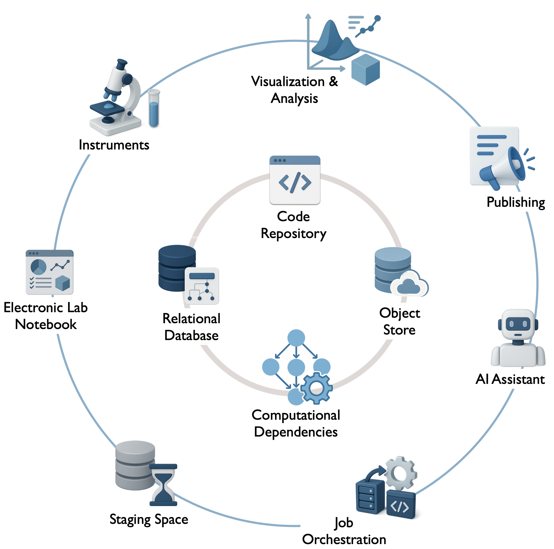 Diagram illustrating the core components defined by the DataJoint standard (inner circle) and the broader ecosystem integration points (outer circle).
These core components, covered by these specifications, include:
Code Repository (e.g., Git): A dedicated version-controlled repository houses each pipeline, including the pipeline definition (schemas, table classes), analysis code, configuration settings, and potentially containerized environments. It serves as the central hub for managing pipeline development, ensuring collaborative development and reproducibility by linking computations to specific code versions.
Relational Database (e.g., MySQL, PostgreSQL): Serves as the pipeline’s metadata store and system of record. It ensures structured tabular storage for experiment data, metadata, and results, enforces data integrity and traceability via foreign-key relationships, and maintains consistency through ACID-compliant transactions.
Computational Dependencies: The encoded logic defining data flow and linking data stages to specific analysis code within the database structure, enabling automation and reproducibility. This transforms the database into a computational engine.
Object Store (Optional but common; e.g., Filesystem, S3, GCS, Azure Blob): A scalable storage backend for managing large scientific datasets (e.g., images, neural recordings, videos) referenced in the relational database but stored externally. This hybrid storage model keeps the database efficient while enabling management of large data objects, often using structured key-naming conventions.
These DataJoint Specs primarily define this core framework and its principles, ensuring that pipelines built using different tools or platforms remain consistent and interoperable. Adherence to this standard is fundamental for achieving data integrity, automated computation, reproducibility, collaboration, and integrated multi-modal data handling.
The current reference implementation for this standard is the open-source DataJoint-Python library datajoint-python, available under the Apache 2.0 License. It provides the essential tools for research teams to build, manage, and integrate their own pipelines using the DataJoint standard.
While the standard defines the core, a fully operational scientific pipeline often integrates with a broader ecosystem (e.g., specific instruments, ELNs, job orchestrators, visualization tools – the outer circle in the diagram). These ecosystem integration points may include:
Job Orchestration: Systems for scheduling, executing, distributing, and monitoring computational jobs (e.g., DataJoint Compute Service, custom scripts, Airflow, SLURM, Kubernetes).
Web Interfaces, APIs, and System Integrations: Tools for interactive data exploration, visualization, data entry (e.g., custom dashboards, JupyterHub), and integration with external systems (ELNs, LIMS, instruments).
While these extensions build upon the core framework, they are generally outside the scope of the base DataJoint specification, allowing flexibility and choice in implementation. Various DIY implementations and commercial offerings may diverge in implementing such extensions.
The DataJoint Platform (not covered by the specs or open standard)
For research teams seeking a fully managed, turnkey solution, DataJoint Inc. offers its Data Operations Platform for Scientific Research. This commercial platform is built upon the open-source core and standards described previously but adds integrated components and services to simplify deployment and reduce operational overhead.
The platform provides a cohesive infrastructure designed to enhance operational excellence in data-intensive research, typically including:
Hosted and managed databases
Integrated, scalable object storage
Automated computation and job orchestration services
Web-based tools for data exploration, visualization, and collaboration
Integration with AI Assistants / LLM agents to potentially assist with tasks like querying, analysis suggestions, or documentation.
Enterprise support, consulting, and training
Pre-integrated functional components (e.g., standard pipelines via the DataJoint Elements program)
Security, compliance, and access control management
The DataJoint Platform aims to provide a reliable, scalable, and secure environment for large-scale scientific workflows, deployable on-premise, in the cloud, or in a hybrid infrastructure.
Crucially, while leveraging the platform’s managed services, research teams retain full ownership and control over their pipeline code and scientific data. This ensures that choosing between a DIY approach with the open-source tools or partnering with DataJoint Inc. for the commercial platform maintains data sovereignty and allows for flexibility and interoperability, grounded in the common DataJoint standard.
Key Objectives and Design Principles
The DataJoint standard is designed around the following key objectives and principles to support robust and scalable scientific data workflows:
Unified Data and Computation: Extend the relational model to a computational database, seamlessly integrating data storage with computational logic and dependencies.
Data Integrity and Reliability: Enforce data validity, consistency, and correctness through rigorous relational database principles, including primary keys, foreign keys, constraints, and ACID-compliant transactions.
Guaranteed Reproducibility: Ensure computations are traceable and reproducible by design, linking results to the exact data, parameters, and code versions used in their generation.
Automation of Computation: Enable intelligent and automated execution of computational steps based on data availability and predefined dependencies.
Seamless Collaboration: Provide a structured, shared “single source of truth” through a common database schema, facilitating concurrent work and consistent data access for teams.
Powerful and Flexible Querying: Leverage the relational model to enable sophisticated and efficient querying of complex datasets based on any recorded attribute.
Integrated Multi-Modal Data Handling: Natively support the management of hybrid datasets, linking structured metadata in the database with large, externally stored data objects (e.g., images, time series, videos).
Scientific Programming Interface: Offer an intuitive interface for scientific programming languages (initially Python) to define schemas, manipulate data, and perform queries without requiring direct SQL composition.
Scalability: Efficiently manage and process large-scale scientific datasets and complex computational workflows.
Extensibility and Interoperability: Allow customization through user-defined data types and facilitate integration with the broader scientific computing ecosystem.
Terminology
DataJoint adopts familiar terms from relational database theory and defines additional terms specific to its computational framework.
| Term | Definition |
|---|---|
| Data Pipeline | A structured system for managing scientific data and computations, encompassing a relational database, code repository, and potentially object storage. It serves as the system of record for a scientific project, enabling structured, reproducible workflows. Also referred to as a DataJoint project or workflow. |
| Computational Database | The core concept where a relational database is extended to treat data and computations jointly, unifying data structures and analysis code to represent and automate entire workflows. |
| Schema | (a) A collection of related table definitions and integrity constraints within the database; (b) A namespace organizing related tables, typically corresponding to a Python module in the code repository. |
| Table | The core relational data structure representing entities or computations. Tables have named and typed attributes and store data as rows. See also Table Tier and Master/Part Table. |
| Attribute (Column/Field) | A named, typed element of a table definition, representing a specific property or data point. Always referenced by name. |
| Row (Record/Tuple) | A single entry (entity instance) in a table, comprising values for each attribute. Rows are uniquely identified by their primary key. |
| Primary Key | A designated set of attributes whose values uniquely identify each row within a table. |
| Foreign Key | A set of attributes in one table that refers to the primary key of another (parent) table, establishing a dependency and enforcing referential integrity. |
| Table Tier | The classification of a table (lookup, manual, imported, computed) indicating its role and how its data is populated (static reference, manual entry, automated import, automated computation). See Table Tiers. |
| Master Table / Part Table | A design pattern where a master table represents a primary entity, and one or more part tables (defined as nested classes) store dependent details. This ensures group integrity, meaning the master and its parts are inserted and deleted together atomically. See Master-Part Relationship. |
make Method | A required method within Computed and Imported table classes that defines the computation or data import process for populating the table’s rows based on upstream data. See Computation. |
| Key Source | For Computed and Imported tables, the set of primary key values from upstream tables for which a computation or import needs to be performed. It identifies the pending tasks for the make method. |
| Query | A function operating on stored or derived data, typically defined via a Query Expression, resulting in a new derived table (relation). |
| Query Expression | A formal definition of a query expressed using DataJoint’s query operators (e.g., restriction &, join *, projection .proj()) acting on tables or other query expressions. |
| Fetch | The execution of a query expression on the database server and the transfer of the resulting data (rows) to the client application. |
| Transaction | A sequence of database operations executed as a single, atomic, consistent, isolated, and durable (ACID) unit. Ensures all operations within the sequence succeed or fail together. |
| Object (Attribute Type) | An attribute type (object) used to store references to large data entities (e.g., files, arrays) managed by DataJoint but typically stored externally in an Object Store rather than directly within the database table row (unlike the blob type). See Object Types. |
| Object Store | A storage backend (e.g., filesystem, S3, GCS) used in conjunction with the relational database to store large data objects referenced by attributes of type object. See Object Storage. |
| Custom Type / Type Adaptor | A user-defined mechanism to handle the conversion between specialized scientific data objects (e.g., specific file formats, complex data structures) and a supported underlying stored attribute type (e.g., blob, object, varchar). See Custom Types. |
Frequently Asked Questions
Is DataJoint an ORM?
Object-Relational Mapping (ORM) is a technique allowing developers to interact with relational databases through object-oriented programming, abstracting direct SQL queries. Popular Python ORMs include SQLAlchemy and Django ORM, often used in web development.
Although DataJoint shares certain ORM characteristics, it is primarily a computational database framework designed explicitly for scientific workflows. Unlike traditional ORMs, which focus mainly on simplifying database interactions for web applications, DataJoint explicitly defines data dependencies and computational relationships, ensuring data integrity, traceability, and reproducibility.
Thus, DataJoint can be considered an ORM specialized for scientific databases, purpose-built for structured experimental data and computational workflows.
Is DataJoint a Workflow Management System?
Not exactly. DataJoint provides robust capabilities for embedding computations within a relational database structure, managing derived data, and tracking explicit data dependencies. However, DataJoint itself does not handle scheduling, distributed execution, or orchestration of parallel computational tasks, which are typical roles of workflow management systems such as Apache Airflow or Nextflow. Instead, DataJoint complements these systems, formalizing data dependencies so that external workflow schedulers can effectively manage computational tasks.
Is DataJoint a Lakehouse?
DataJoint and lakehouses share some similar goals—such as integrating structured data management with scalable storage and computational capabilities. However, a lakehouse typically merges the flexibility of data lakes (handling raw, semi-structured data at scale) with the structured schemas and transactional guarantees of traditional databases.
In contrast, DataJoint focuses specifically on scientific data workflows, emphasizing rigorous schema definitions, explicit computational dependencies, and robust data integrity. While lakehouses offer flexible analytics on structured and unstructured data, DataJoint prioritizes precise data modeling, reproducibility, and computational traceability within structured scientific datasets.
Therefore, DataJoint complements lakehouse architectures but is tailored specifically for managing structured experimental data and computational pipelines in science.
Does DataJoint require SQL knowledge?
No, DataJoint does not require SQL knowledge, but understanding relational concepts can be helpful.
DataJoint provides a Python-based API that abstracts SQL, allowing users to define schemas, insert data, and query tables without writing SQL. Instead of composing SQL queries, users interact with the database using intuitive Python methods.
Examples comparing SQL vs. DataJoint
| SQL | DataJoint-Python |
|---|---|
CREATE TABLE | Define tables as Python classes |
INSERT INTO | .insert() method |
SELECT * FROM ... | .fetch(), .proj(), .aggr() |
JOIN | table1 * table2 |
WHERE ... | table & condition |
Since DataJoint uses relational database backends, all data can be accessed through SQL as well.
Pipeline Design
A data pipeline within the DataJoint framework is a structured system designed to manage scientific data, its inherent dependencies, associated computations, and execution workflows.
Pipeline ≡ Python Package
A DataJoint pipeline SHALL be implemented as a dedicated Python package. Within this package, Python modules correspond to database schemas. This architectural convention ensures that data, computations, and their interdependencies are organized, traceable, and reproducible.
A DataJoint pipeline adheres to a Directed Acyclic Graph (DAG) structure, wherein:
Nodes represent Python modules, which in turn correspond to database schemas.
Edges represent dependencies between these modules. These dependencies include:
Standard Python import dependencies between modules.
Referential dependencies between tables across different schemas (bundles of foreign keys dependencies), which define the data flow and relational structure of the pipeline.
Constraint: Acyclicity of Dependencies
Cyclical dependencies are strictly prohibited at multiple levels:
All referential constraints (foreign keys) within a single schema MUST form a DAG.
The dependencies between schemas (formed by foreign keys linking tables in different schemas, and by Python import statements between modules) MUST also collectively form a DAG.
This ensures a unidirectional flow of data and computational dependencies throughout the pipeline.
Database Schema ≡ Python Module
Each database schema in a DataJoint pipeline SHALL correspond to a distinct Python module. This module serves as a namespace for organizing a collection of logically related tables. Adherence to a one-to-one mapping between database schemas and Python modules promotes modularity and maintainability of the pipeline code.

Key principles of this mapping include:
Database Schemas: Function as containers for groups of logically related tables within the relational database.
Python Modules: Structure the pipeline’s Python code into modular and scalable units, each representing a database schema.
Intra-Schema Dependencies: Foreign key relationships between tables within the same schema MUST also form a DAG, reinforcing a unidirectional data dependency flow at the schema level.
This structured correspondence between the database organization and the codebase ensures synchronization, thereby facilitating reproducibility, collaboration, and long-term maintenance.
Database Table ≡ Python Class
In the DataJoint framework, each database table SHALL be represented by a Python class. A consistent naming convention MUST be followed to map Python class names to database table names:
| Python Construct | Database Construct |
|---|---|
| Class Names | Written in CamelCase |
| Table Names | Written in snake_case |
| Fully Qualified Python Class Name | <module>.<ClassName> |
| Fully Qualified Database Table Name | <schema_name>.<table_name> |
Example Mapping:
Python Class:
scan.ScanLocationDatabase Table:
scan.scan_location
This naming convention ensures clarity, consistency, and unambiguous alignment between the Python implementation of the pipeline logic and the underlying relational database schema.
Table Tiers
Each table within a DataJoint pipeline SHALL be assigned to one of four predefined tiers. These tiers classify tables based on their role and the method by which their data are populated and maintained. In graphical representations of the pipeline (e.g., diagrams generated by dj.Diagram), distinct color codes are conventionally used to visually differentiate these tiers:
| Tier | Description | Color Code (in Diagrams) |
|---|---|---|
lookup | Static reference data that is part of the schema definition (e.g., parameters, controlled vocabularies). | Gray |
manual | Data manually entered from external sources, typically by users. | Green |
imported | Data automatically ingested from external sources (e.g., raw data files, external databases). | Blue |
computed | Data generated from upstream tables through automated computations. | Red |
Note on Color Codes: Standard GitHub Flavored Markdown (GFM) does not support the direct rendering of colored text. However, these color codes are a standard convention used in DataJoint’s graphical schema visualization tools (e.g.,
dj.Diagramoutputs) and MAY be applied in other documentation formats that support rich text styling, such as HTML or LaTeX.
The classification of tables into these tiers provides a clear conceptual separation between manually curated data, externally sourced data, and computationally derived data. This distinction is fundamental to maintaining data integrity, provenance, and understanding the data flow within the pipeline.
Table Definition
The definition of a table in DataJoint specifies its structural and functional characteristics within the pipeline. Each table definition encompasses the following elements:
Table Name: The identifier for the table, defined as a Python class name and translated into a corresponding database table name according to specified naming conventions.
Table Tier: The classification of the table (e.g.,
lookup,manual,imported,computed) which dictates its role and data population method, as defined in Table Tiers.Attributes: A set of named columns, each with a defined data type, an optional default value, and an optional descriptive comment. These define the data structure of the table.
Primary Key: A designated set of attributes whose combined values uniquely identify each row within the table.
Foreign Keys: References to primary keys in other (parent) tables, establishing relational dependencies and ensuring referential integrity.
Indexes: Additional database indexes (beyond those implicitly created for primary and foreign keys) to optimize query performance or enforce uniqueness constraints on non-primary key attributes.
A common method for specifying these elements is through a multi-line string assigned to a class attribute named definition within the table’s Python class declaration.
Example: Basic Table Definition Structure
@schema # Decorator associating the class with a DataJoint schema object
class TableName(dj.Table): # Base class depends on the table tier
    definition = """
    # A descriptive comment for the table
    primary_key_attribute_1 : type       # Comment for attribute 1
    primary_key_attribute_2 : type       # Comment for attribute 2
    ---                                  # Primary key separator
    secondary_attribute_1   : type       # Comment for attribute 3
    secondary_attribute_2   : type = default_value # Attribute with a default
    -> ParentTable                       # Foreign key definition
    index (secondary_attribute_1)        # Secondary index definition
    """
While the definition string is a prevalent convention, alternative programmatic methods for defining table structures MAY be supported by specific DataJoint client implementations, provided they ultimately resolve to these fundamental elements.
Attribute Definition
Each attribute in a table definition SHALL be specified by its name, data type, an optional default value, and an optional comment. The syntax for defining an attribute within the definition string is:
attribute_name : type[ = default_value][ # comment]
Where:
attribute_name: A valid identifier for the attribute.type: A DataJoint-supported Attribute Type.default_value(optional): A literal value to be used if no value is provided for this attribute during data insertion.A special default value of
nullexplicitly declares the attribute as nullable. An attribute without a default value is implicitly NOT NULL, unless it is part of a nullable foreign key. Primary key attributes SHALL NOT be nullable.
comment(optional): A human-readable description of the attribute, typically preceded by a#character.
Examples of Attribute Definitions:
experiment_id   : int unsigned       # Unique identifier for the experiment
recording_date  : date               # Date of data recording
notes           : varchar(1000) = '' # Optional notes, defaults to empty string
analysis_param  : float = null       # A nullable analysis parameter
Primary Key
Every table in a DataJoint pipeline MUST have a primary key. The primary key is a set of one or more attributes whose collective values uniquely identify each row in the table.
Specification: Attributes constituting the primary key SHALL be listed first in the table
definitionstring, appearing above a mandatory primary key separator line, which consists of three hyphens (---).Composition:
A primary key MAY consist of a single attribute (simple primary key).
A primary key MAY consist of multiple attributes (composite primary key).
A primary key MAY be empty (i.e., consist of zero attributes), defining a “singleton table.” A singleton table can contain at most one row.
Constraints:
Primary key attributes SHALL NOT have default values.
Primary key attributes SHALL NOT be nullable.
Example: Primary Key Definition
    definition = """
    subject_id    : varchar(32)   # Part 1 of the composite primary key
    session_id    : uint16        # Part 2 of the composite primary key
    ---                           # Primary key separator
    session_date  : date
    experimenter  : varchar(64)
    """
In this example, (subject_id, session_id) jointly form the primary key.
Schema Normalization
Tables within a DataJoint pipeline SHOULD be designed according to the principles of database normalization. The objective is to ensure that each table represents a single, well-defined entity type or relationship.
Entity Integrity: Each row in a table corresponds to a unique instance of the entity type that the table represents, uniquely identified by its primary key.
Attribute Relevance: All non-key attributes within a table MUST directly describe a property of the entity identified by the primary key.
Minimizing Redundancy: Schema normalization aims to reduce data redundancy and improve data integrity by decomposing tables that represent multiple entity types or contain repeating groups of information into several, appropriately linked tables.
Adherence to normalization principles facilitates data consistency, reduces anomalies during data modification, and improves the overall clarity and maintainability of the pipeline schema.
Foreign Keys
A foreign key establishes a referential link between a “child” table (the table containing the foreign key definition) and a “parent” table (the table referenced by the foreign key). This link ensures **referential integrity, meaning that rows in the child table can only reference existing rows in the parent table.
Foreign keys SHALL be defined on separate lines within the definition string of the child table, using the -> operator to point to the Python class name of the parent table.
Syntax for Foreign Key Definition
-> ParentClassName
-> [modifier[, modifier...]] ParentClassName
-> [modifier[, modifier...]] ParentClassName.proj(new_name1=old_name1, ...)
Where:
ParentClassName: The Python class name of the parent table being referenced.modifier(optional): Keywords such asnullableoruniquethat alter the properties of the foreign key attributes inherited into the child table or the constraint itself.nullable: If specified, the foreign key attributes inherited into the child table’s primary key become nullable if they are part of the child’s primary key. If they are secondary attributes in the child, they are nullable if the parent’s corresponding primary key attributes allow it or if the FK itself is marked nullable. This allows a child record to exist without referencing a parent record.unique: If specified, creates a unique constraint on the foreign key attributes in the child table, ensuring a one-to-one or one-to-zero-or-one relationship from the parent to the child.
.proj(new_name=old_name, ...)(optional): A projection clause that allows renaming of the primary key attributes inherited from theParentClassName. This is useful if the default inherited names would conflict with existing attributes in the child table or if different naming is preferred.
Constraints:
Cyclical dependencies created by foreign keys are strictly prohibited. The collective graph of all foreign key relationships within and between schemas MUST be a Directed Acyclic Graph (DAG).
A foreign key in DataJoint MUST reference the entirety of the primary key of the parent table. Referencing a non-primary key set of attributes or a subset of the parent’s primary key is not permitted by this specification.
Effects of a Foreign Key Definition:
Attribute Inheritance: The primary key attributes of the
ParentClassNameare implicitly included in the attribute set of the child table if they are not already present. Their data types and properties (e.g., nullability, if modified) are derived from the parent’s primary key.Referential Constraint: A referential integrity constraint is established in the database, ensuring that values in the foreign key attributes of the child table must match existing primary key values in the
ParentClassName.Implicit Index: An index is automatically created on the foreign key attributes in the child table to optimize join operations and referential integrity checks.
Indexes and Unique Constraints
Beyond the implicit index created for the primary key, tables MAY define additional secondary indexes to optimize query performance or enforce uniqueness constraints on non-primary key attributes or combinations thereof.
Secondary Index: Speeds up data retrieval operations that filter or sort by the indexed attribute(s). Defined using the syntax:
index (attribute_name_1, attribute_name_2, ...)Unique Index: Enforces that the combination of values in the indexed attribute(s) is unique across all rows in the table. Defined using the syntax:
unique index (attribute_name_1, attribute_name_2, ...)
Example: Table with Secondary and Unique Indexes
@schema
class Person(dj.Manual):
    definition = """
    # Table representing a person with unique identifiers
    person_id        : uint32      # Unique person identifier (Primary Key)
    ---
    first_name       : varchar(50)
    last_name        : varchar(50)
    drivers_license  : varchar(20) = null
    cell_phone       : varchar(15) = null
    email            : varchar(100) = null

    index (last_name, first_name)  # Secondary index for faster name searches
    unique index (drivers_license) # Ensures driver's license is unique (if not null)
    unique index (cell_phone)      # Ensures cell phone is unique (if not null)
    unique index (email)           # Ensures email is unique (if not null)
    """
This definition facilitates efficient searches by (last_name, first_name). The unique indexes ensure data integrity for drivers_license, cell_phone, and email.
Note on Nullable Unique Constraints: A unique index on an attribute that permits
NULLvalues allows multiple rows to containNULLin that attribute, asNULLis generally not considered equal to anotherNULLfor constraint purposes. The exact behavior MAY depend on the underlying database system (e.g., MySQL, PostgreSQL).
Lookup Tables
Lookup tables (dj.Lookup tier) store static or semi-static reference data that is considered an integral part of the pipeline’s schema definition rather than dynamic experimental data. Examples include controlled vocabularies, lists of experimental parameters, or standardized codes.
Content Definition: The initial content of a lookup table SHALL be provided as part of its class definition, typically via a class attribute named
contents. This ensures that a new deployment of the pipeline will have these tables pre-populated with their defined reference data.Mutability: While initially defined with the schema, the contents of lookup tables MAY be updated or extended over the lifecycle of the pipeline, reflecting an evolution of the reference data. Such changes are typically managed as schema migrations or controlled updates.
Example: ChemicalElement Lookup Table
import datajoint as dj

schema = dj.Schema('chemistry') # Assumes 'schema' is a dj.Schema() object

@schema
class ChemicalElement(dj.Lookup):
    definition = """
    # Lookup table for chemical elements
    atomic_number : uint8       # Atomic number (Primary Key)
    ---
    symbol        : char(2)     # Chemical symbol
    name          : varchar(20) # Element name
    atomic_weight : decimal(7,4)  # Standard atomic weight
    """
    contents = [
        {'atomic_number': 1, 'symbol': 'H',  'name': 'Hydrogen',  'atomic_weight': 1.008},
        {'atomic_number': 2, 'symbol': 'He', 'name': 'Helium',    'atomic_weight': 4.0026},
        {'atomic_number': 3, 'symbol': 'Li', 'name': 'Lithium',   'atomic_weight': 6.94},
        # ... additional elements
    ]
Attribute Types
DataJoint defines a standardized, concise set of fundamental attribute types for use in table definitions.
These types abstract the underlying SQL data types provided by supported relational database backends (e.g., (PostgreSQL and MySQL)), offering a consistent interface tailored for scientific data workflows.
This specification prioritizes type names that are intuitive to users in scientific computing environments (e.g., uint8 rather than SQL’s TINYINT UNSIGNED).
Core Attribute Types
The following core attribute types SHALL be supported by DataJoint implementations:
| Category | Type | Description |
|---|---|---|
| UUID | uuid | Universally Unique Identifier (RFC 4122). Default values are not supported for uuid attributes. |
| Integers | int8, uint8, int16, uint16,int32, uint32, int64, uint64 | Standard signed and unsigned integer types of varying bit widths. |
| Floating-Point | float32, float64 | Single-precision (32-bit) and double-precision (64-bit) floating-point numbers. Note: NaN (Not a Number) behavior MAY vary by backend; e.g., MySQL does not natively support NaN in indexed FLOAT columns. |
| Decimal | decimal(M,N) | Fixed-point decimal number with a total precision of M digits and N digits after the decimal point (scale). |
| Character Strings | char(N), varchar(N) | Fixed-length (char) or variable-length (varchar) character strings, where N specifies the maximum length. |
| Enumeration | enum('val1', 'val2', ...) | A type restricted to a predefined set of allowed string values. |
| Date | date | Represents a calendar date (year, month, day) in ISO 8601 format (YYYY-MM-DD). A special default value of NOW MAY be used to set the current date upon insertion. |
| Time / Timestamp | timestamp | Represents a point in time, typically with microsecond precision, stored in UTC. Values SHOULD conform to ISO 8601 format. A special default value of NOW MAY be used to set the current timestamp upon insertion. |
| Binary Large Object | blob | Stores large binary data directly within the database row (inline storage). Suitable for moderately sized binary objects. |
| Object Reference | object | Stores a reference (e.g., a key or path) to an external data object managed by DataJoint but stored outside the primary database (e.g., in an object store or file system). See Object Types. |
| Custom Type | <adaptor_name> | A user-defined type managed by a Custom Type Adaptor, allowing for specialized storage and handling of complex data structures. |
Distinction: blob vs. object Attribute Types
The blob and object types both handle non-scalar data, but differ in their storage strategy and typical use cases:
| Type | Intended Use | Data Storage Location |
|---|---|---|
blob | Raw binary data stored directly within the database table row. Suitable for relatively small to moderately sized binary data where inline storage is acceptable and efficient. | Database System (e.g., as BLOB or BYTEA columns in MySQL/PostgreSQL). |
object | References to data entities stored externally to the primary database. Suitable for large files, datasets, or complex objects where external storage is preferred for scalability or management. | External Storage Systems (e.g., file systems, cloud object stores like S3/GCS/Azure Blob, network-attached storage). The database stores metadata and a reference key. |
Object Types (External Storage)
DataJoint pipelines often employ a hybrid storage model to manage large-scale scientific datasets efficiently. In this model:
The relational database serves as the central repository for structured metadata, relational dependencies, and transaction management.
An external object store is utilized for handling large, often unstructured or semi-structured, scientific data objects such as images, multidimensional arrays, videos, or specialized file formats.
This approach leverages the strengths of relational databases for data integrity and querying, while utilizing the scalability and cost-effectiveness of dedicated object storage solutions for bulk data.
How object Attributes Work
The object attribute type facilitates this hybrid model by enabling object-augmented schemas. Tables can include attributes of type object, which store references to data entities residing in an external store. These externally stored objects are:
Managed by DataJoint: Their lifecycle (insertion, retrieval, deletion) is integrated with DataJoint operations.
Referenced via Keys: Stored and retrieved using a structured key-naming convention or path, ensuring unambiguous linkage.
Tracked with Metadata: The relational database stores metadata associated with each external object, such as its format, size, checksum, and version, facilitating efficient management and validation.
The dj.Object Interface for Custom Object Handling
To enable DataJoint to manage custom external object types, users MAY define Python classes that subclass dj.Object. Such classes MUST implement a specific interface to handle the serialization, storage, retrieval, and verification of these objects.
The required methods for a dj.Object subclass are:
| Method Signature | Description |
|---|---|
put(self, store, key: str) -> dict | Writes the instance’s data to the specified store (a configured object storage backend) under the given key (a unique identifier or path). Returns a dictionary of metadata (e.g., checksum, version, timestamp) to be stored in the database. |
get(cls, store, key: str) -> "dj.Object" | A class method that reads data from the store using the key and reconstructs an instance of the dj.Object subclass. |
get_meta(self) -> dict | Returns a dictionary of metadata about the object instance (e.g., size, checksum, version), typically reflecting the state as stored or to be stored. |
verify(self, store, key: str) -> bool | Confirms that the object corresponding to key exists in the store and is valid (e.g., by checking its checksum or integrity). Returns True if valid, False otherwise. |
Metadata for External Objects
For each attribute of type object, DataJoint (or the custom dj.Object implementation) SHALL ensure that relevant metadata is stored within the relational database alongside the reference. This metadata typically includes:
Object Key/Path: The unique identifier or path used to locate the object in the external store.
File Format/Extension: The storage format of the object (e.g.,
.zarr,.tiff,.nwb).Size: The size of the object in bytes.
Checksum: A hash (e.g., MD5, SHA256) of the object’s content for data integrity verification.
Version (optional): A version identifier if the object undergoes versioning.
Timestamp (optional): Timestamps for creation or last modification.
Custom Types (Type Adaptors)
Custom types, also known as type adaptors, extend DataJoint’s native type system to allow seamless integration and management of diverse scientific data structures as if they were standard attributes stored directly in database columns. They provide a mechanism for converting between complex Python objects or specialized file formats and one of DataJoint’s Core Attribute Types suitable for database storage.
DataJoint projects MAY define and register a collection of custom type adaptors tailored to their specific data handling needs.
Functionality of Custom Types:
Enable the use of complex or non-standard data types within DataJoint tables while preserving database integrity and queryability.
Define bidirectional conversion logic:
Transforming user-provided objects into a storable format upon insertion.
Reconstructing the original (or equivalent) Python objects from the stored format upon retrieval.
Abstract storage details from the user, providing a consistent interface for data interaction.
Key Benefits:
Extends DataJoint’s data modeling capabilities to a wide range of scientific data formats.
Ensures compatibility with the relational storage model for complex data.
Simplifies the handling (insertion, fetching) of specialized objects for end-users.
Can facilitate backward compatibility with legacy data representations.
Implementation and Registration:
Type adaptors SHALL be implemented as Python classes subclassing from dj.CustomType. These classes MUST implement the following methods and properties:
type_name(property): A string representing the unique name by which this custom type is referenced in table definitions (e.g.,<my_custom_type>).stored_type(property): A string specifying the underlying DataJoint Core Attribute Type (e.g.,blob,object,varchar(255), or another registered<adaptor_name>) used for actual storage in the database.put(self, user_object: object) -> object: Converts theuser_object(the Python object provided during insertion) into thestored_typeformat. Thekeyargument (representing the primary key of the record being inserted) MAY be optionally accepted byputif its values are needed for the conversion or storage process (e.g., for constructing object paths ifstored_typeisobject).get(self, stored_object: object) -> object: Converts thestored_object(data retrieved from the database instored_typeformat) back into the user-level Python object. Thekeyargument MAY be optionally accepted bygetif needed for reconstruction.
Custom type adaptors MUST be accessible (e.g., imported) and registered with the DataJoint client (e.g., via a plugin mechanism or explicit registration call like dj.register_type(MyCustomAdaptor)) before any schemas using these types are declared or activated. Revisions to type adaptors SHOULD maintain backward compatibility to ensure existing data remains accessible and correctly interpretable.
Example Type Adaptors:
type_name | stored_type | Purpose |
|---|---|---|
<dj_blob> | blob | Serializes arbitrary Python objects into a generic blob format, often used for backward compatibility with older DataJoint blob storage. |
<zarr_array> | object | Manages a NumPy array stored externally as a Zarr dataset, referenced by a path/key. |
<tif_image> | object | Manages an image stored externally as a TIFF file. |
Usage in Table Definition:
Once registered, a custom type adaptor is used in a table definition string by its type_name.
class ProcessedData(dj.Computed):
    definition = """
    -> upstream.Analysis
    ---
    computed_matrix : <zarr_array>    # Uses the <zarr_array> custom type
    result_summary  : <dj_blob>       # Uses the <dj_blob> custom type
    """
During an insert operation, DataJoint will invoke the put method of the corresponding registered adaptor for attributes of custom types. During a fetch operation, the get method will be invoked.
Master-Part Relationship
The master-part relationship is a design pattern in DataJoint used to enforce group integrity, ensuring that a primary entity (the “master”) and its dependent components (the “parts”) are managed as a single atomic unit. This is crucial for scenarios where multiple related records must always exist together or not at all.
Ensuring Group Integrity
Consider a scenario where an experimental trial (master) produces multiple simultaneously recorded data streams (parts). The master-part pattern ensures that the trial record and all its associated data stream records are inserted together, and if the trial record is deleted, all its data stream records are also automatically deleted.
Master-Part Pattern Definition
Master Table: A standard DataJoint table of any tier that represents the primary entity.
Part Table(s): Tables that store dependent details or components of the master entity. Part tables SHALL be defined as nested classes within the Python class definition of their master table.
The fully qualified Python class name for a part table follows the format: module_name.MasterClassName.PartClassName. The corresponding database table name will also reflect this nested structure (e.g., <schema_name>.<master_table_name>__<part_table_name>).
A part table MUST always have a foreign key referencing its master table. To simplify this declaration, DataJoint provides the alias -> master within the definition string of a part table. This alias automatically establishes the foreign key relationship to the enclosing master table, inheriting its primary key attributes.
Restrictions on Master-Part Relationships
No Nested Masters: A part table SHALL NOT itself serve as a master table for other part tables. The master-part relationship is limited to one level of nesting.
Exclusive Master: A part table SHALL belong to exactly one master table. It cannot have multiple master tables.
Hierarchical Data: For more complex hierarchical relationships extending beyond a single master-part level, multiple distinct master tables, each potentially with their own part tables, SHOULD be used, linked by standard foreign key relationships.
Example: Cell Segmentation with Master-Part
@schema
class Segmentation(dj.Computed):  # Master table
    definition = """
    -> acq.Image
    -> seg.SegmentationMethod
    ---
    segmented_image_object : <image_object_type> # Reference to the full segmented image
    region_count           : uint16              # Number of segmented regions
    """

    class Region(dj.Part):  # Part table, nested within Segmentation
        definition = """
        # Stores individual segmented regions for each Segmentation entry
        -> master             # Foreign key to the Segmentation master table
        region_idx : uint16   # Differentiates regions within the same segmentation
        ---
        region_pixels_object : <region_mask_object_type> # Object with pixel data for the region
        region_area          : float                     # Area of the region
        """
Key Characteristics of this Example:
Atomic operations: An entry in
Segmentationand all its correspondingSegmentation.Regionentries are inserted or deleted as a single transaction.Referential integrity: No
Segmentation.Regionentry can exist without a valid parentSegmentationentry.Simplified definition: The
-> masteralias clearly defines the link to the master table.
Enforcement via Transaction Processing
The DataJoint framework guarantees the integrity of master-part relationships through its transaction handling:
Atomic Insertion: When records are inserted into a master table that has associated part tables, the master record and all its corresponding part records (often provided together in a single structured dictionary or object) MUST be inserted within a single database transaction. If any part of the insertion fails, the entire transaction is rolled back.
Cascaded Deletion: When a record in a master table is deleted, all corresponding records in its part tables SHALL be automatically deleted by the database system due to the cascading nature of the foreign key constraint.
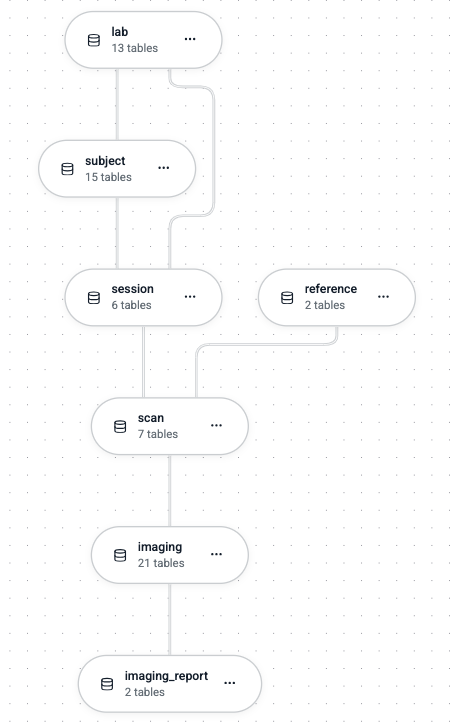
Diagram
DataJoint comes with a formally-defined diagramming notation implemented by the dj.Diagram class.
The pipeline is visualized as a Directed Acyclic Graph with nodes corresponding to classes and edges corresponding to foreign key dependencies between them.
The tables are grouped by their schemas, which, in turn, also form a DAG, where edges bundle all the foreign key from the child schemas to the parent schemas.
The diagram is always depicted with the data moving top-to-bottom (foreign keys referencing upward) or left-to-right (foreign keys referencing leftward).
dj.Diagram are graph objects that support an algebra of graph operations: union, intersection, and dilation.
The nodes are colored according to their table tier.
Object Storage
DataJoint integrates object storage into its relational database-driven pipelines to efficiently manage large scientific datasets. Object storage is used for two primary purposes:
Object-Augmented Schemas – Storing large, unstructured data (e.g., images, time series) externally while keeping structured metadata in the database.
Database Backup & Export – Providing a structured, shareable repository of pipeline data.
Object-Augmented Schemas
A DataJoint pipeline follows a hybrid storage model, where:
The relational database manages structured metadata, dependencies, and transactions.
The object store handles large, unstructured scientific data (e.g., images, multidimensional arrays).
This scalable approach maintains fast querying, data integrity, and transactional consistency, while enabling flexible, distributed storage of large datasets.
Storage Backend Configuration
A DataJoint client is configured to access the storage backend associated with each database. Supported backends include:
Local storage – POSIX-compliant file systems (e.g., NFS, SMB).
Cloud-based object storage – Amazon S3, Google Cloud Storage, Azure Blob, MinIO.
Hybrid storage – Combining local and cloud storage for flexibility.
DataJoint uses fsspec to ensure compatibility across multiple storage backends.
Example Structured Storage Pattern
A DataJoint project creates a structured hierarchical storage pattern:
📁 project_name/
├── datajoint.toml
├──📁 schema_name1/
├──📁 schema_name2/
├──📁 schema_name3/
│  ├── schema.py
│  ├── 📁 tables
│  │   ├── table1/key1-value1.parquet
│  │   ├── table2/key2-value2.parquet
│  │   ...
│  ├── 📁 objects
│  │   ├── table1-field1/key3-value3.zarr
│  │   ├── table1-field2/key3-value3.gif
...  ...
When using object storage, the corresponding keys might be:
s3://project_name/schema_name3/objects/table1/key1-value1.parquet
s3://project_name/schema_name3/fields/table1-field1/key3-value3.zarr
The organizational structure of stored objects is configurable, allowing partitioning based on primary key attributes.
Example configuration in datajoint.toml:
# Configuration for object storage
[object_storage]
partition_pattern = "subject{subject_id}/session{session_id}"
This structure dynamically replaces placeholders {subject_id} and {session_id} with actual values.
Example Stored Objects with Partitioning
s3://my-bucket/project_name/subject123/session45/schema_name3/objects/table1/key1-value1/image1.tiff
s3://my-bucket/project_name/subject123/session45/schema_name3/objects/table2/key2-value2/movie2.zarr
This structured naming approach allows:
Efficient indexing & retrieval using key-based lookups.
Scalable organization across flat object storage systems.
Cross-platform compatibility with both file systems & cloud storage.
Export, Sharing, and Backup/Restore
The structured project data repository serves as a comprehensive, publishable copy of the dataset, accessible by DataJoint and other tools.
Designed for human navigation & automated tools.
Supports exporting portions of the dataset (specific tables, time ranges).
Enables easy backup & migration of scientific workflows.
The export method recreates the data repository in full at another location. DataJoint offers tools to restore the database from the file repository using the tabular data, supporting data publishing and pipeline cloning alongside the data.
Data Operations
Data operations alter the state of the data stored in the database.
Records (rows) in a stored table are considered immutable: each is inserted or deleted as a whole using insert and delete operators.
However, to allow correcting errors in existing data, the update1 operator is provided to perform deliberate corrections in the data by changing the values of individual attributes.
Insert comes in three flavors:
insert1(record)for inserting an individual recordinsert(sequence)for batches of recordsinsert(query_expression)for inserting query results
Insert1
The method Table.insert1(rec) inserts one record rec into one table.
The record to be inserted must be fully formed and comply with all data integrity constraints:
All attributes must be of the right data type, i.e. must meet attribute domain constraints specified in the table definition.
The record must provide values for all required fields.
Unique constraints must be satisfied (no duplicate values).
Referential integrity must be upheld (foreign keys must reference existing records).
If the record violates any constraints, the operation fails, ensuring atomicity—either the record is successfully inserted, or nothing is changed.
A record value may be specified as an ordered tuple, in which case all fields must be present, or as a mapping (dict), in which case optional fields may be omitted.
Example:
# insert a student record
Student.insert1({
    'student_id': 1002,
    'first_name': 'Alice',
    'last_name': 'Johnson',
    'sex': 'F',
    'date_of_birth': '1998-03-12',
    'home_address': '1234 Elm Street',
    'home_city': 'Springfield',
    'home_state': 'IL',
    'home_zipcode': '62704',
    'home_phone': '(217)555-1234'
})
Batch Insert
The method Table.insert(seq) inserts a sequence of records.
In this case, the entire sequence of records is inserted in a single transaction: if a single record fails to insert, the entire sequence fails.
This makes the insert operator atomic.
Example:
Student.insert([
    {'student_id': 1000, 'first_name': 'Rebecca', 'last_name': 'Sanchez',
     'sex': 'F', 'date_of_birth': '1997-09-13',
     'home_address': '6604 Gentry Turnpike Suite 513',
     'home_city': 'Andreaport', 'home_state': 'MN',
     'home_zipcode': '29376', 'home_phone': '(250)428-1836'},
    {'student_id': 1001, 'first_name': 'Matthew', 'last_name': 'Gonzales',
     'sex': 'M', 'date_of_birth': '1997-05-17',
     'home_address': '1432 Jessica Freeway Apt. 545',
     'home_city': 'Frazierberg', 'home_state': 'NE',
     'home_zipcode': '60485', 'home_phone': '(699)755-6306x996'}
])
Query Insert
The method Table.insert(query_expression) inserts the result of a query expression.
In this case, the query expression is treated similarly to the inserted sequence in batch insert and must meet the same requirements.
The remarkable property of query insert is that no data is fetched to the client. Both the source query expression and the subsequent insert are performed server-side as an atomic transcation without sending data to the client. Both the query and the insert are performed as an atomic transaction.
Example:
# insert all possible majors for all students
StudentMajor.insert(Department.proj() * Student.proj())
Delete
The delete operation removes records from stored tables with cascading effects to all dependent records. Delete is often used in combination with the restriction operator to specify records to delete.
Example:
# delete all students
Student.delete()

# delete specific students
(Student & "student_id IN (500, 501, 503)").delete()
Delete cascades to all dependent records in the downstream tables after proper user confirmation.
Update
Update is used to change the values of secondary attributes in one record only.
The Table.update1(rec) operator takes a mapping, rec, which must provide:
The complete value of the primary key for the updated record
The new values for all updated attributes
Example:
# Update email and cellphone for student id 1001
Student.update1({
    'student_id': 1001,
    'email': 'new_email@example.com',
    'cell_phone': '(555)123-4567'
})
Note that this formulation is incapable of updating primary key attributes. The record must already exist and only secondary attributes will be updated. Modifying the primary key requires deleting and reinserting the record.
Effect of Foreign Key Constraints
Foreign keys enforce referential integrity, which affects how insert, delete, and update1 operations behave:
Insert: When using
insertorinsert1, foreign key constraints require that referenced records exist in the parent table before dependent records can be added. This ensures that no orphaned entries are created. If a foreign key references a non-existent record, the insertion will fail. This rule helps maintain consistency by preventing invalid references in dependent tables.Delete: On deletion (
delete), foreign keys enforce cascading behavior, meaning that deleting a referenced record automatically removes all dependent records downstream. This prevents data inconsistencies by ensuring that no dependent records exist without their required parent records.Update: For updates,
update1modifies secondary attributes of a single record. An update can fail if the secondary attribute is part of a foreign key and no matching record is found in the parent table.Drop: When a table is dropped from the schema, all dependent tables will be dropped as well. The DataJoint client provides a full list of tables to be dropped before executing the schema update.
Queries
A query is a server-side operation on stored or derived data that yields a new derived table. The results of a query are transferred to the client application through fetch operations.
Query Expressions
A query expression is the formal definition of a query. It is constructed by applying Query Operators to one or more input tables (or the results of other query expressions) to define an output table. Query expressions in DataJoint adhere to the following principles:
Composable: Query expressions can be combined, allowing the output of one expression to serve as an input for another, enabling the construction of complex queries from simpler components.
Declarative: Query expressions specify the desired data to be retrieved rather than the explicit sequence of computational steps to obtain it. The DataJoint client and underlying database engine are responsible for optimizing and executing the query.
Relational: The result of any query expression is a well-formed relational table, possessing a defined set of attributes and a primary key, thus maintaining relational integrity.
Fetch Operations
Fetch operations execute a query expression on the database server and transfer the resulting data to the client application.
.fetch() Method
The .fetch() method retrieves all rows satisfying the query expression.
Function: Executes the query and returns the complete result set.
Output Formats: The result set can be returned in various formats, including but not limited to a sequence of dictionaries, a NumPy structured array, or a Pandas DataFrame, depending on client implementation and configuration.
Example:
# Retrieve all attributes for students residing in California.
query_ca_students = Student & "home_state = 'CA'"
results = query_ca_students.fetch()
# 'results' contains the fetched data.
.fetch1() Method
The .fetch1() method retrieves a single row satisfying the query expression.
Function: Executes the query and returns one row.
Constraints: This method SHALL raise an error if the query result contains zero rows or more than one row.
Output Format: The result is typically a dictionary representing the single row.
Example:
# Retrieve attributes for the student with student_id = 1002.
query_student = Student & "student_id = 1002"
try:
    student_record = query_student.fetch1()
    # 'student_record' contains the data for the specified student.
except dj.DataJointError as e:
    # Handle error if student is not found or if multiple records exist.
    print(f"Query execution error: {e}")
Iteration over Query Results
DataJoint query expression objects SHALL be iterable. Iteration allows for row-by-row processing of query results.
Function: Enables sequential processing of result rows, typically fetching data incrementally from the server. This approach is memory-efficient for large result sets.
Output per Iteration: Each iteration SHALL yield a dictionary representing a single row from the query result.
Example:
# Process records for students residing in Texas.
query_tx_students = Student & "home_state = 'TX'"
for record in query_tx_students:
    # 'record' is a dictionary for the current student row.
    process_student_record(record) # Example processing function
Query Operators
DataJoint provides a set of fundamental query operators for constructing query expressions. These operators act on tables or query expressions to produce new tables.
The primary query operators are:
Restriction and Anti-Restriction:
&and-Projection:
.proj(...)Join:
*Aggregation:
.aggr(...)Union:
+
These operators can be combined. Standard Python operator precedence SHALL apply, and parentheses () MAY be used to explicitly control the order of evaluation.
Operator: Restriction (&, -)
The restriction operator filters the rows of a table based on specified conditions. It is expressed in two forms:
A & condition: Selects rows from tableAthat satisfy thecondition.A - condition: Selects rows from tableAthat do not satisfy thecondition(anti-restriction).
Algebraic Closure under Restriction: The primary key and attribute set of the resulting table are identical to those of the operand A. The entity type is preserved.
Forms of Restriction Conditions:
Restriction by a Condition String: Conditions are often expressed as SQL-like predicate strings.
# Select students from California.
ca_students = Student & "home_state = 'CA'"

# Select students not from California.
non_ca_students = Student - "home_state = 'CA'"
Restriction by a Dictionary: Conditions can be specified as a dictionary mapping attribute names to values. These imply equality conditions.
# Students from Texas (dictionary form).
tx_students = Student & {'home_state': 'TX'}
Restriction by a Sequence of Conditions (Logical OR): When a query is restricted by a sequence (e.g., a list) of condition strings, the conditions SHALL be combined using logical OR (disjunction).
# Select students who are from outside California OR were born on or after January 1, 2010.
selected_students = Student & ["home_state <> 'CA'", "date_of_birth >= '2010-01-01'"]
Restriction by Conjunction (Logical AND): To combine conditions using logical AND (conjunction), conditions MAY be applied sequentially or by using a
dj.AndListobject.# Select young students from outside California (sequential application). young_non_ca_students = (Student & "home_state <> 'CA'" & "date_of_birth >= '2010-01-01'") # Equivalent using dj.AndList. young_non_ca_students_alt = Student & dj.AndList([ "home_state <> 'CA'", "date_of_birth >= '2010-01-01'" ])Restriction by a Subquery: The result of another query expression can be used as a condition. The restriction acts as a semijoin (for
&) or an anti-semijoin (for-).# Select students enrolled in course 'CS101'. cs101_enrollments = Enroll & "course_id = 'CS101'" students_in_cs101 = Student & cs101_enrollments # Select students not enrolled in course 'CS101'. students_not_in_cs101 = Student - cs101_enrollmentsRestriction by
dj.Top(Limiting Results): Thedj.Topoperator limits the number of rows returned.# Select the first 5 students (order is undefined unless specified). top_5_students = Student & dj.Top(5) # Select the 5 students with the most recent birth dates (youngest). youngest_5_students = Student & dj.Top(5, order_by="date_of_birth DESC")
Operator: Projection (.proj())
The projection operator selects a subset of attributes from a table. It can also be used to rename attributes and compute new attributes derived from existing ones.
Attribute Selection:
# Select first_name, last_name, and email attributes from the Student table.
student_contacts = Student.proj('first_name', 'last_name', 'email')
Attribute Renaming:
# Select first_name and last_name, renaming them to 'first' and 'last' respectively.
renamed_student_names = Student.proj(first='first_name', last='last_name')
Primary Key Preservation: The primary key attributes of the operand table SHALL always be included in the result of a projection, even if not explicitly specified. Primary key attributes MAY be renamed.
# This projection returns only the primary key attributes of the Student table.
student_primary_keys = Student.proj()
Computed Attributes: New attributes can be computed using expressions that operate on the operand’s attributes. The expressions are typically database functions.
# Compute 'full_name' and 'age'.
student_derived_info = Student.proj(
    full_name='CONCAT(first_name, " ", last_name)',
    # Example age calculation (exact function varies by SQL dialect)
    age='TIMESTAMPDIFF(CURDATE(), date_of_birth) / 365.25'
)
# Result includes primary key attributes, full_name, and age.
Inclusion/Exclusion of Attributes: The ellipsis (
...) denotes all attributes of the operand. It MAY be used with subtraction (-) to exclude specific attributes.# Select all attributes from Student except 'email'. students_no_email = Student.proj(..., -'email')
Algebraic Closure under Projection: The primary key of the resulting table is identical to that of the operand A. The entity type is preserved.
Operator: Join (*)
The join operator A * B combines rows from table A and table B. The operation first forms the Cartesian product of the rows and then restricts the result to rows where attributes common to both A and B satisfy Semantic Matching conditions.
Usage:
# Combine Student information with their Enrollment records.
student_enrollments = Student * Enroll

# Combine Enrollment records with Course details.
# Assumes Enroll references Course via a foreign key on course_id.
enrollment_course_details = Enroll * Course
Algebraic Closure under Join: The entity type and primary key of the join result depend on the functional dependencies between the operands A and B with respect to the join attributes.
* If one operand is functionally dependent on the other across the join attributes (e.g., B’s attributes in the join are determined by A’s primary key), the resulting entity type is that of the determining operand (A), and its primary key is preserved as the result’s primary key.
* If the operands are functionally independent with respect to the join, the resulting entity type represents a pairing of the two entities, and the primary key of the result is typically the union of the primary keys of A and B (excluding redundant attributes from the shared join columns).
Operator: Aggregation (.aggr())
The aggregation operator A.aggr(B, computed_attributes...) projects attributes from table A (similar to A.proj()) and, additionally, computes new attributes by applying aggregation functions to groups of data from table B. Rows in B are grouped according to the primary key of table A.
Requirements:
Tables
AandBMUST be semantically compatible for the attributes involved in forming the groups.Table
BMUST contain all attributes constituting the primary key of tableA, with identical names and compatible types, to allow grouping ofB’s rows byA’s primary key.
Conceptual SQL Equivalence: The operation is analogous to a
LEFT JOINfromAtoB(onA’s primary key), followed by aGROUP BYclause onA’s primary key, with aggregation functions applied to attributes fromB.Usage:
# For each student, compute their full name and average grade.
student_summary = Student.aggr(
    Grade,                                  # Table B, providing data for aggregation
    full_name='CONCAT(first_name, " ", last_name)', # Projected/computed from A
    avg_grade='AVG(grade)'                  # Aggregated from B
)
Algebraic Closure under Aggregation: The primary key and entity type of the resulting table A.aggr(B, ...) are identical to those of table A.
Operator: Union (+)
The union operator A + B combines rows from table A and table B.
Requirements for Operands:
Semantic Compatibility: All attributes shared between
AandBMUST be semantically compatible.Primary Key Congruence: Tables
AandBMUST have the same primary key attributes (identical names, types, and semantic meaning). They must represent the same entity type.
Behavior:
If
AandBonly contain primary key attributes, the result is the set-theoretic union of the rows.If
AandBcontain secondary attributes, the result includes all primary key entries present in eitherAorB. All unique secondary attributes from bothAandBare included in the result schema. If both operands possess a secondary attribute with the same name for a given primary key entry, the value from the left operand (A) SHALL be used in the result.
Usage:
# Combine CurrentStudent and FormerStudent records.
all_students = CurrentStudent + FormerStudent
Algebraic Closure under Union: The primary key and entity type of the resulting table are identical to those of the operands A and B.
Semantic Matching
For binary operators that combine two tables A and B (e.g., join *, restriction by subquery A & B_query, aggregation A.aggr(B, ...), union A + B), a mechanism is required to match rows between A and B. DataJoint employs a rule termed semantic matching.
Semantic matching between rows of tables A and B is performed as an equality condition on all pairs of attributes that satisfy both:
The attributes have the same name in both
AandB.The attributes trace to the same original attribute definition through an uninterrupted chain of foreign keys.
This rule is more restrictive than the NATURAL JOIN in SQL, which typically only requires attributes to have the same name. The DataJoint approach prevents accidental matching of attributes that are homonymous but semantically distinct.
If tables A and B possess attributes with identical names that do not satisfy the second condition (i.e., they do not share the same lineage), these attributes are considered to “collide.” Such a semantic mismatch renders the binary operator invalid, and an error SHALL be raised. To resolve semantic mismatches, the projection operator (.proj()) MUST be applied to one or both operands to rename or remove the colliding attributes prior to the binary operation.
Example of Semantic Mismatch: Given
Student(student_id, name)andCourse(course_id, name). The attributenamecollides.# Invalid operation due to 'name' collision. # Student * CourseResolution:
# Rename 'name' in Course to 'course_name' before joining.
valid_join = Student * Course.proj(course_name='name')
# Resulting attributes include 'name' (from Student) and 'course_name'.
Algebraic Closure
A fundamental property of DataJoint’s query system is algebraic closure. This means that the result of any valid query expression is itself a well-formed relational table. This output table:
Possesses a defined set of named attributes with known data types.
Has a well-defined primary key.
Maintains the lineage of its attributes, tracing back to their original definitions. This persistence of lineage is crucial for enabling subsequent Semantic Matching.
The principle of algebraic closure allows complex queries to be constructed by composing simpler query expressions, where the output of one operation serves as a valid input for the next. Each operator section above specifies how the primary key and entity type of its result are determined, preserving this closure.
Universal Sets (dj.U())
Universal sets, denoted by dj.U(...), are symbolic constructs representing the set of all possible values for a specified list of attributes, or a singular universal context if no attributes are specified. They are not directly fetchable tables but serve as operands in query expressions.
dj.U('attr1', 'attr2', ...): Represents a conceptual table containing all possible combinations of values for the attributes'attr1','attr2', etc.dj.U(): Represents a singular entity, effectively a table with no attributes and one conceptual row. This is primarily used for universal aggregations.
Applications of Universal Sets
Projecting Unique Values: When restricted by an existing table,
dj.U(<attributes>)combined with that table results in the distinct values of<attributes>present in the table.# Retrieve all unique last names from the Student table. unique_last_names = dj.U('last_name') & Student # Retrieve all unique full names from the Student table. unique_full_names = dj.U('first_name', 'last_name') & StudentUniversal Aggregation:
dj.U()(with no arguments) serves as the grouping entity for aggregations that span all rows of a table, rather than grouping by the primary key of another table.# Count the total number of students. total_student_count = dj.U().aggr(Student, n_students='COUNT(student_id)') # The result is a table with one row and one attribute 'n_students'. # The primary key of this result is the empty set.Aggregation by arbitary groupings:
dj.U(<attribites>)creates a new grouping entity with an arbitrary primary key for use in aggregations for which no existing entity type fits that purpose.# count how many students were born in each year and month student_counts = dj.U('year_of_birth', 'month_of_birth').aggr( Student.proj( year_of_birth='YEAR(date_of_birth)', month_of_birth='MONTH(date_of_birth)'), n_students='COUNT(*)' )In this case, the rules os semantic matching are lifted.
Computation
DataJoint integrates computation as an intrinsic component of its data model.
Certain tables, designated as auto-populated (i.e., dj.Imported or dj.Computed tiers), represent the results of computations rather than directly ingested data.
The population of these tables is governed by methods defined within their corresponding class definitions.
Key characteristics of automated computation in DataJoint include:
Restricted Manual Insertion: Users SHALL NOT manually insert data into auto-populated tables.
Automated Result Generation: Data in these tables are generated exclusively through predefined computational logic.
Cascaded Execution: The introduction of new data or dependencies in upstream tables MAY trigger the automated computation of dependent results in downstream auto-populated tables.
This model is designed to ensure data consistency, integrity, and computational reproducibility throughout the data pipeline.
The make Method: Defining Computational Logic
Auto-populated tables (i.e., tables of tier dj.Imported or dj.Computed) MUST implement a method named make, which encapsulates the logic for populating a single entry (or a master entry and its associated part entries) in the table.
Method Signature:
def make(self, key, **make_opts) -> None:The key argument is a dictionary representing a single primary key value from the table’s key source, identifying the specific entity for which the computation is to be performed.
Optional make_opts MAY be passed to customize the behavior of the make method.
The execution of a make method for a given key typically involves three principal steps:
Fetch Data: Retrieve necessary input data from upstream (parent) tables, restricted by the provided key.
Compute Results: Process the fetched data to generate the required output values for the attributes of the current table and its part tables (if any).
Insert Results: Store the computed results into the current table (and its part tables, if applicable) using the
self.insert1()method (andself.Part.insert()for any Part tables). The inserted record MUST include the attributes from the input key along with the newly computed attributes.
Example: Computing an Average Signal
@schema
class SignalAverage(dj.Computed):
    definition = """
    -> RawSignal
    ---
    avg_signal: float
    """

    def make(self, key: dict) -> None:
        # Step 1: Fetch input data from upstream table.
        raw_signal_value = (RawSignal & key).fetch1("signal")

        # Step 2: Compute the result.
        average_signal_value = raw_signal_value.mean()

        # Step 3: Insert the computed result.
        self.insert1({**key, "avg_signal": average_signal_value})
This structured approach ensures that all computed data are traceable to their inputs and the specific computational logic applied.
Each invocation of the make method for a single key SHALL be executed within a single, ACID-compliant database transaction. This guarantees:
Computational Integrity: Results are correctly and uniquely associated with their specific set of inputs defined by
key.Atomic Execution: The entire operation (fetch, compute, insert for the given
key) either completes successfully, or, in case of an error, no partial data is persisted in the database, maintaining a consistent state.
Handling Long-Running Computations
For computations that are expected to be long-running (potentially hours or days), maintaining an open database transaction for the entire duration of the make method can lead to operational issues, such as blocking other database operations or exceeding transaction timeout limits.
To address this, DataJoint supports a deferred transaction verification mechanism. This involves separating the data fetching and computation from the final data insertion and verification, minimizing the duration of the database transaction. This is achieved by implementing three distinct methods instead of a single make method:
make_fetch(self, key: dict) -> object:Retrieves all necessary input data from the database based on
key.This method executes outside the main insertion transaction.
The returned
fetched_dataobject is passed tomake_compute.
make_compute(self, key: dict, fetched_data: object) -> object:Performs the primary computation using the
fetched_data.This method executes outside any database transaction.
The returned
computed_resultsobject is passed tomake_insert.
make_insert(self, key: dict, fetched_data: object, computed_results: object) -> None:This method executes within a minimal database transaction.
Prior to calling
make_insert, DataJoint SHOULD re-fetch the input data (by callingmake_fetcha second time) to verify that inputs have not been modified since the initial fetch.If inputs are verified to be consistent, DataJoint calls
make_insert.If inputs have changed, the transaction SHOULD be rolled back, and the entire computation is cancelled for subsequent retries.
The same example from above will appear as follows:
Example: Computing an Average Signal with short transaction time -- three-part make method
@schema
class SignalAverage(dj.Computed):
    definition = """
    -> RawSignal
    ---
    avg_signal: float
    """

    def make_fetch(self, key: dict) -> None:
        # Step 1: Fetch input data from upstream table.
        raw_signal_value = (RawSignal & key).fetch1("signal")
        return raw_signal_value,


    def make_compute(self, key: dict, fetched: tuple) -> tuple:
        raw_signal_value, = fetched
        # Step 2: Compute the result.
        average_signal_value = raw_signal_value.mean()
        return average_signal_value,

    def make_insert(self, key: dict, fetched: tuple, computed: tuple) -> None:
        average_signal_vaue, = computed
        # Step 3: Insert the computed result.
        self.insert1({**key, "avg_signal": average_signal_value})
An alternative implementation of this three-part make method is to convert a normal make method into a generator yielding the fetched data and computed results. This effectively implements the three-part make method, but is more succinct.
The example below illustrates this approach:
Example: Computing an Average Signal with short transaction time -- Generator Implementation
@schema
class SignalAverage(dj.Computed):
    definition = """
    -> RawSignal
    ---
    avg_signal: float
    """

    def make(self, key: dict) -> None:
        # Step 1: Fetch input data from upstream table.
        raw_signal_value = (RawSignal & key).fetch1("signal")
        computed = yield raw_signal_value,   # yield the fetched data and receive computed results

        if computed is None:
            # Step 2: Compute the result.
            average_signal_value = raw_signal_value.mean()
            computed = average_signal_value,
            yield computed  # yield the computed results

        # Step 3: Insert the computed result.
        average_signal_value, = computed
        self.insert1({**key, "avg_signal": average_signal_value})
        yield  # signals the end of computation
DataJoint’s internal logic will automatically call the three methods in the correct order, as illustrated in the pseudocode below: Pseudocode for Deferred Transaction Handling:
fetched = self.make_fetch(key)
computed = self.make_compute(key, fetched)

<begin transaction>
fetched_again = self.make_fetch(key)

if fetched != fetched_again:   # peforms a deep comparison of the two tuples
    <rollback transaction>
else:
    self.make_insert(key, fetched, computed)
    <commit transaction>
This strategy minimizes the time database locks are held, at the cost of fetching input data twice.
It is recommended for computations where the computation time significantly exceeds the data fetching time.
It is the user’s responsibility to segregate the functionality into the three distinct parts (all fetches in make_fetch, all computations in make_compute, and all inserts in make_insert). However, in future standards, DataJoint may enforce this segregation.
Key Source: Determining Entries for Computation
The key source for an auto-populated table defines the set of primary key values for which the make method needs to be executed. DataJoint automatically determines the key source.
Formation: The key source is derived from the join of all parent tables referenced by foreign keys present in the primary key definition of the auto-populated table. Only the primary key attributes of these parent tables are projected.
Exclusion: Entries for which data already exists in the auto-populated table are excluded from the key source. This ensures that computations are performed only for new or missing entries.
Example: Key Source for a Computed Table
Consider a computed table ProcessedImage that processes images recorded by different methods:
@schema
class ProcessedImage(dj.Computed):
    definition = """
    -> acq.Image
    -> ProcessingMethod
    ---
    processed_data: blob
    """
The key source in this case is:
acq.Image.proj() * ProcessingMethod.proj() - ProcessedImageThis expression identifies all combinations of Image and ProcessingMethod primary keys that do not yet have a corresponding entry in ProcessedImage.
Computed vs Imported Tables
Auto-populated tables are primarily categorized into two tiers: dj.Computed and dj.Imported.
The distinction lies in the origin of their input data and the implications for reproducibility:
| Tier | Purpose | Reproducibility | Data Source |
|---|---|---|---|
Computed (dj.Computed) | Fully reproducible computations | ✅ Guaranteed | Uses only pipeline data |
Imported (dj.Imported) | Data ingested from external sources | ❌ Not guaranteed | Reads from external sources (e.g., instruments, APIs) |
While both tiers use the make (or make_fetch/make_compute/make_insert) method for populating entries, dj.Computed tables are designed to ensure that, given the same upstream pipeline data and the same computational code, the results are identical. dj.Imported tables introduce external dependencies, meaning reproducibility also relies on the stability and versioning of these external sources.
Summary of automated computing
DataJoint integrates computation directly into its data model, similar to how spreadsheets update formulas when inputs change.
Computation tables (
ComputedandImported) must define amake(self, key)method to handle data processing.The key source automatically determines which entries need computation.
Computed tables ensure full reproducibility, while imported tables depend on external sources.
For long-running computations, DataJoint supports transaction handling to prevent database locking, where the
makemethod needs to be split into three parts:make_fetch,make_compute, andmake_insert.DataJoint ensures atomic transaction processing, preventing incomplete computations.
By structuring computation within DataJoint pipelines, researchers can build efficient, reproducible, and scalable data workflows.